贝叶斯推理

任务场景

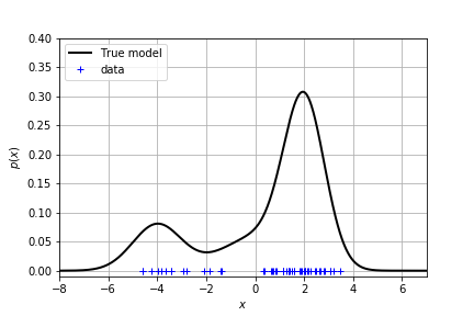
给定数据，真实的分布是未知的。我们学习的任务就是去拟合出真实的分布。现在我们给出一个真实分布是 GMM，在上面采样得到一组数据。你是否能够根据数据去拟合出这个分布？

GMM(means, variances, weights)
true_model = models.GMM([-4, 0, 2], [1, 2, .7], [0.2, 0.2, 0.6])

单峰分布

用高斯分布拟合

我们知道高斯分布是长这样的

$$\DeclareMathOperator{\Norm}{\mathcal{N}} \DeclareMathOperator{\Gam}{Gam} \DeclareMathOperator{\e}{exp} p(x \mid \mu, \sigma^2) = \Norm(x \mid \mu, \sigma^2) = \frac{1}{\sqrt{2\pi\sigma^2}} \e\{ \frac{-(x - \mu)^2}{2\sigma^2} \}$$

• $\mu$ is the mean of the Gaussian density
• $\sigma^2$ is the variance of the Gaussian density
• $\lambda = \frac{1}{\sigma^2}$ is the precision of the Gaussian density

（等等我们可以用 $\lambda$ 代替方差来写高斯分布）

为了估计真实的分布，可以采用最大化似然的办法得到均值和方差

$$\begin{align} \mu &= \frac{1}{N} \sum_i x_i \\ \sigma^2 &= \frac{1}{N} \sum_i x_i^2 \end{align}$$

N = len(X)
mean = np.sum(X)/N
var = np.sum(X**2)/N

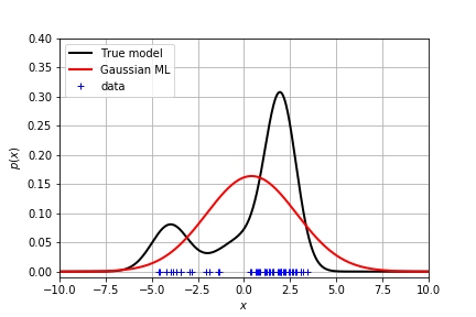
显然这个结果不能很好地拟合真实分布。

贝叶斯推理：加入均值和方差的先验

A common and convenient choice of prior for the Gaussian is the Normal-Gamma prior:

$$p(\mu, \lambda \mid m_0, \kappa_0, a_0, b_0) = \Norm(\mu \mid m_0, (\kappa_0 \lambda)^{-1}) \Gam(\lambda \mid a_0, b_0)$$

where:

$$\Gam(\lambda \mid a_0, b_0) = \frac{1}{\Gamma(a_0)} b_0^{a_0} \lambda^{a_0 - 1} \e \{ -b_0 \lambda\}$$

$m_0$, $\kappa_0$, $a_0$ and $b_0$ are called hyper-parameters. They are the parameters of the prior distribution.

为了对 Normal-Gamma 分布有个形象的了解，可以绘图看到，它的均值和方差是服从这样的概率分布的

NormalGamma(mean, kappa, a, b)
ng_prior = models.NormalGamma(0, 2, 5, 6)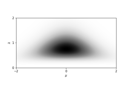

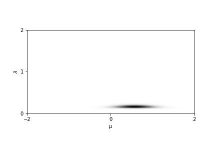
由于 Normal-Gamma 是 正态分布的 共轭先验，因此 Normal-Gamma 的后验有闭式解，且可以写成如下形式：

$$p(\mu, \lambda \mid \mathbf{x}) = \Norm(\mu \mid m_n, (\kappa_n \lambda)^{-1}) \Gam(\lambda \mid a_n, b_n)$$

where:

$$\begin{align} m_n &= \frac{\kappa_0 m_0 + N \bar{x}} {\kappa_0 + N} \\ \kappa_n &= \kappa_0 + N \\ a_n &= a_0 + \frac{N}{2} \\ b_n &= b_0 + \frac{N}{2} ( s + \frac{\kappa_0 (\bar{x} - m_0)^2}{\kappa_0 + N} ) \\ \bar{x} &= \frac{1}{N} \sum_i x_i \\ s &= \frac{1}{N} \sum_i (x_i - \bar{x})^2 \end{align}$$

$N$ is the total number of point in the the training data and $m_n$, $\kappa_n$, $a_n$ and $b_n$ are the parameters of the posterior. Note that they are different from the hyper-parameters !!

因此加入后验的影响后，均值和方差的分布成为更加聚集的一小团。

当需要做预测任务时，则需要把均值和方差边缘化（积分掉），得到数据分布。恰好这个分布是学生分布。由此可以得到每个数据点的概率密度：

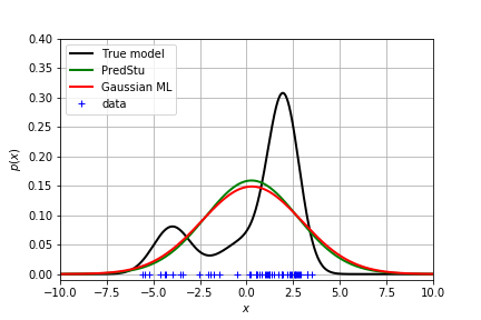
但是由于是单峰的，拟合效果还是很差！

多峰分布

用高斯混合模型拟合

我们尝试用 K 个不同的高斯分布来拟合真实分布：

$$p(x|\boldsymbol{\mu}, \boldsymbol{\lambda}, \boldsymbol{\pi}) = \sum_{k=1}^{K} \pi_k \Norm(x|\mu_k, (\lambda_k)^{-1})$$

• $\boldsymbol{\mu}$ is the vector of $K$ means
• $\boldsymbol{\lambda}$ is the vector of $K$ precisions
• $\boldsymbol{\pi}$ is the vector of $K$ weights such that $\sum_{k=1}^K \pi_k = 1$

其中给不同高斯加的权重作为隐变量。

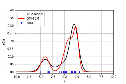
用 EM 算法求解参数

• initialize the parameters of the GMM
• iterate until convergence ($\log p(\mathbf{x} | \theta^{new}) - \log p(\mathbf{x} | \theta^{old}) \le 0.01$):
  • Expectation (E-step): compute the probability of the latent variable for each data point
  • Maximization (M-step): update the parameters from the statistics of the E-step.

具体推导可以看 Expectation Maximization algorithm 以及 GMM

last_llh = -1e8
while 1e-2 < np.absolute(llh - last_llh):
    # E-step
    Z = gmm.EStep(X)
    
    # M-step
    gmm.MStep(X, Z)
    
    last_llh = llh
    llh = gmm.logLikelihood(X)
    print('log-likelihood:', llh)

具体的 EStep 和 MStep 可以看这里

不同的参数初始化得到的效果不同。这里给出了一个拟合得较好的分布：

贝叶斯推理：加入先验

加入参数的先验：

$$\DeclareMathOperator{\Dir}{Dir} p(\boldsymbol{\pi}) = \Dir(\boldsymbol{\pi} \mid \boldsymbol{\alpha}_0)$$ $$p(\mu_k, \lambda_k) = \Norm(\mu_k \mid m_0, (\kappa_0 \lambda_k)^{-1}) \Gam(\lambda_k \mid a_0, b_0)$$

如果仍旧想用 EM 算法求解参数，则在 M 步会直接把均值和方差算出来，而不是算出均值和方差的后验。因此不能用 EM 算法。

考虑到参数之间有相互依赖的关系，可以用 Gibbs Sampling 得到参数的后验分布。给出以下三个条件分布，在每次迭代中，都假设知道了条件值，采出样本。最终它们将趋向于真实分布。

latent variable $z_i$

$$\begin{align} p(z_i \mid \mathbf{x}, \Theta) &= p(z_i \mid x_i, \boldsymbol{\pi}, \boldsymbol{\mu}, \boldsymbol{\lambda}) \\ p(z_i = k \mid x_i, \boldsymbol{\pi}, \boldsymbol{\mu}, \boldsymbol{\lambda}) &= \frac{\pi_k \Norm(x_i \mid \mu_k, \lambda_k)} {\sum_{j=0}^{K} \pi_j \Norm(x_i \mid \mu_j, \lambda_j)} \end{align}$$

mean and variance

We define the set of all data point $x_i$ that are assigned to the component $k$ of the mixture as follows:

$$\mathbf{x}_{(k)} = \{ x_i : z_i = k, \forall i \in \{1,... , N \} \}$$

and similarly for the latent variables $\mathbf{z}$:

$$\mathbf{z}_{(k)} = \{ z_i : z_i = k, \forall i \in \{1,... , N \} \}$$ $$\begin{align} p(\mu_k, \lambda_k \mid \mathbf{x}, \mathbf{z}, \Theta_{\smallsetminus \{ \mu_k, \lambda_k \} } ) &= p(\mu_k, \lambda_k \mid \mathbf{x}_{(k)}, \mathbf{z}_{(k)}, \Theta_{\smallsetminus \{ \mu_k, \lambda_k \} } ) \\ &= \Norm(\mu_k \mid m_{n,k}, (\kappa_{n,k} \lambda_k)^{-1}) \Gam(\lambda_k \mid a_{n,k}, b_{n,k}) \end{align}$$

where:

$$\begin{align} m_{n,k} &= \frac{\kappa_0 m_0 + N_k \bar{x}_k} {\kappa_0 + N_k} \\ \kappa_{n,k} &= \kappa_0 + N_k \\ a_{n,k} &= a_0 + \frac{N_k}{2} \\ b_{n,k} &= b_0 + \frac{N_k}{2} ( s + \frac{\kappa_0 (\bar{x}_k - m_0)^2}{\kappa_0 + N_k} ) \\ N_k &= \left\vert \mathbf{x}_{(k)} \right\vert \\ \bar{x}_k &= \frac{1}{N_k} \sum_{\forall x \in \mathbf{x}_{(k)}} x \\ s_n &= \frac{1}{N} \sum_{\forall x \in \mathbf{x}_{(k)}} (x_i - \bar{x})^2 \end{align}$$

NOTE: these equations are very similar to the Bayesian Gaussian estimate. However, it remains some difference

weights

$$\begin{align} p( \boldsymbol{\pi} \mid \mathbf{x}, \mathbf{z}, \Theta_{\smallsetminus \{ \boldsymbol{\pi} \} } ) &= p( \boldsymbol{\pi} \mid \mathbf{z}) \\ &= \Dir(\boldsymbol{\pi} \mid \boldsymbol{\alpha}) \end{align}$$

where:

$$\alpha_{n,k} = \alpha_{0,k} + N_k \; ; \; \forall \, k = 1\dots K$$

for i in range(20):
    # Sample the latent variables
    Z = bgmm.sampleLatentVariables(X)
    
    # Update the parameters
    bgmm.sampleMeansVariances(X, Z)
    bgmm.sampleWeights(Z)
    
    # Just for plotting, this is not part of the Gibbs Sampling algorithm.
    plotting.plotGMM(bgmm.gmm, fig=fig, ax=ax, color='b', lw=.5, label='sampled GMM')

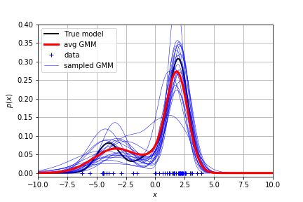
每次迭代的参数都可以生成一条蓝线。把蓝线加权平均得到了红线。看起来还是比较接近真实分布的。

相关教程

• Introduction To Bayesian Inference (jupyter notebook)
• Gibbs sampling for fitting finite and infinite Gaussian mixture models